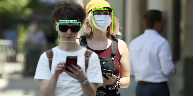
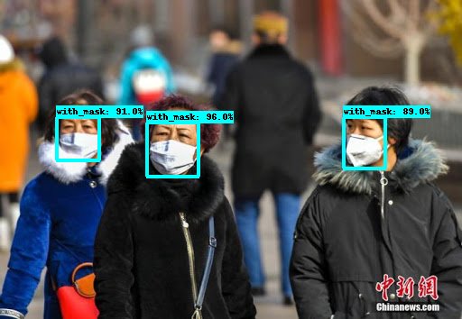
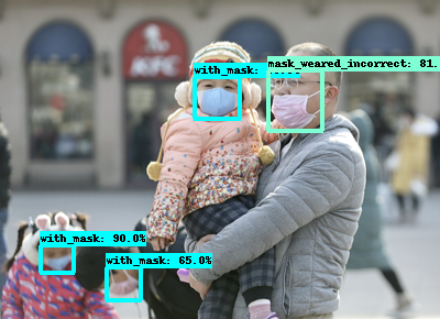
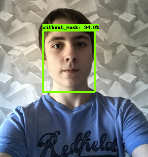
We will build a custom Object Detection Model to perform Face Mask Detection using Tensorflow Object Detection API to detect people with and without a mask in a given image or video stream or webcam. We will use Kaggle’s Face Mask Detection dataset for this purpose. The dataset contains 853 images with 3 classes: with mask, without_mask and incorrect mask (mask_weared_incorrect). The dataset includes annotations for all the classes.
The final release of Tensorflow 2 has been around since September 2019. This came with many new upgrades to Tensorflow 1.x but due to the differences in their working, many legacy codes require migrating to Tensorflow 2. One of the most requested repositories to be migrated to Tensorflow 2 was the Tensorflow Object Detection API which took over a year for release, providing minor compatible supports over time. However, on 10th July 2020, Tensorflow Object Detection API released official support to Tensorflow 2.0.
The release introduced new object detection architectures: CenterNet and EfficientDet, supported only by the TF2 version of the repository. They also added new pre-trained weights for COCO (a common dataset to test object detection models on) models that can be used for fine-tuning our custom datasets. For this tutorial, we will be using EfficientDet D0 – one of the new additions to the object detection models. To read in-depth about EfficientDet, you can read the paper published.
Introduction to Object Detection
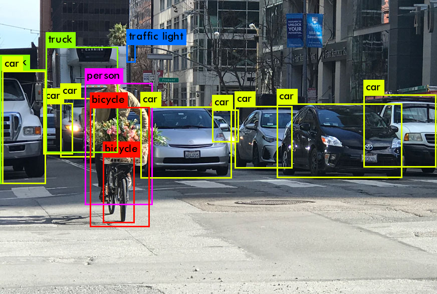
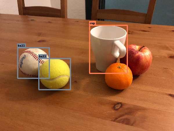
Object Detection is the process of finding a particular object (instance) in a given image frame using image processing techniques. Such techniques deal with videos by treating them as multiple image frames. There are various approaches and architectures to choose from; to name a few: Faster R-CNN and SSD are widely used in various applications. If you’re new to the terms, it can be considered as a program that uses a technique to detect your objects, wherein each technique has its pros and cons. However, we highly recommend reading more about the architectures as it will help you understand how they work, which can enable you to consistently build efficient models.
Before we begin
Defining the problem
- Create your Problem Statement: Find out what do you want to detect.
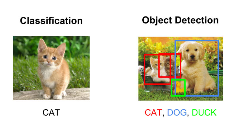
- Object Detection vs Image Classification: This is a major question, whether you want to detect some objects in a random image, or do you want to classify the image given a particular structure of the image. i.e. If you have portrait photos of animals and you want to see if it is a dog or a cat, the problem is classification-based. On the other hand, if you have an image with multiple animals in the same image, you’re better off using Object Detection to detect all cats and dogs in the image. If you’re here looking for Image Classification, follow our guide on “How To Build a Cat vs Dog Image Classifier using CNN” [Link]
Choosing Data and Model
- Finding the dataset: Object Detection heavily relies on data. The more the data (good quality data), the better the results will be. It is very likely to find a common dataset on various platforms like:
- Kaggle
- Google Datasets
- Github
However, in case you are looking to detect an object that does not have a dataset readily available, you may need to take the pain to click various images of the object in different conditions, from different angles. The more the images, the better. We recommend having at least 200-300 images per class for any detection task.
- Annotate the dataset (if not done already): Annotation refers to the Region of Interest (ROI) for a particular object or class in a given image. In our case, the dataset we’re using already has annotated the classes in XML files. However, if your dataset does not have annotations, you can use various tools available. We would recommend using LabelImg (we do not promote the tool)
- Selecting the model: While some architectures provide great accuracy, they consume a lot of resources (for training as well as testing). Whereas some models provide very quick results at the cost of having a lower accuracy. ED-7x is one of the top object detection models as of writing the blog. However, we do not need to use a high resource-based model for our simple task of detecting face masks (also, the free GPU on colab cannot train an ED7). We will start with the basic model, EfficientDet-0. For a complete list of models supported by Tensorflow-2 Object Detection API, you can visit the detection zoo page for Tensorflow2. You can use any model of your choice; however, the configuration might be different for each one. We, for this tutorial, are using EfficientDet D0 512×512.
Installing Tensorflow Object Detection API on Colab
All the steps are available in a Colab notebook that is linked to refer and run the code snippets directly. You can find the notebook here. The notebook also consists of few additional code blocks that are out of the scope of this tutorial.
- Setup the Colab: Once we have all the required data available, we can now get into the coding action. You can make your notebook or directly run the notebook available. Before starting, change the Runtime Type to GPU to use the free GPU provided by Colab. Training a model on GPU speeds up the process greatly.
- Clone our repository Tensorflow-Object-Detection: It contains few utility files that we’ll use for data preparation and inference:
!git clone https://github.com/deepme987/Tensorflow-Object-Detection- Clone the tensorflow-models repository: It contains the required files for Object Detection. After cloning the repository, we install the package and run the test code. In case you wish to go through the package installation code, it is referred from Tensorflow API. If the test runs without any errors, you’ve successfully built the package.
!pip install pip --upgrade %cd /content !git clone --quiet https://github.com/tensorflow/models.git %cd /content/models/research/ !protoc object_detection/protos/*.proto --python_out=. %cp object_detection/packages/tf2/setup.py . !python -m pip install --use-feature=2020-resolver . !python object_detection/builders/model_builder_tf2_test.py %cd /content/Tensorflow-Object-Detection- Download the data from Kaggle and upload on Colab. Alternatively, you can setup Kaggle on Colab (code included in the notebook) and download directly on the notebook to avoid downloading and uploading from your machine (recommended for large datasets or slow connections).
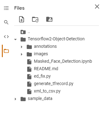
- Extract the dataset in the repository directory. At this stage, your directory should look as follows:
Preparing the data
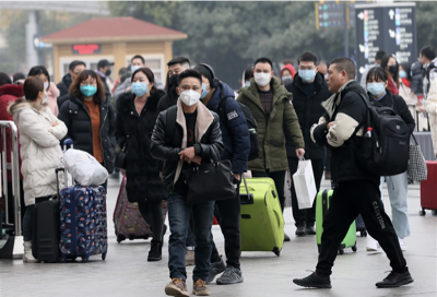
Before we dive into the data, we can manually open a few images to view the dataset. Below are few images available in our dataset


The annotations provided in the dataset are in xml format. However, we need to convert them to csv (comma-separated values) file. We’ve included a script to convert annotations from xml to csv in the repository.
!python xml_to_csv.py --xml_path=annotations/ --csv_output=annotations.csvAfter converting annotations to csv, we need to split the data into train and test. This can be achieved using sklearn’s GroupShuffleSplit. We split data at 70-30, you may edit this by changing the test_size value in GroupShuffleSplit. The grouped data is then saved as csv as train_labels.csv and test_labels.csv which we’ll use to create TFRecords.
Note: We cannot use train_test_split for this case as multiple fields can refer to object in the same image. In such case, we will have same image in the train as well as the test sets, but with different object instance. Hence, we use GroupShuffleSplit to group based on the filename of the images.
import pandas as pd
data = pd.read_csv("annotations.csv")

from sklearn.model_selection import GroupShuffleSplit
train_inds, test_inds = next(GroupShuffleSplit(test_size=0.30, random_state = 7).split(data, groups=data['filename']))

train = data.iloc[train_inds]
test = data.iloc[test_inds]

train.to_csv("train_labels.csv")
test.to_csv("test_labels.csv")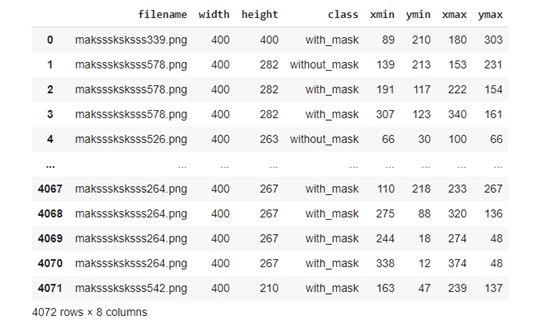
Create a file named labelmap.pbtxt on your editor (for users referring to Colab Notebook, this step is available in a code block). This file consists of IDs starting from 1 and its corresponding class label. This is necessary as Tensorflow understands numeric values and not string classes. For our case, the classes are mask, without_mask, mask_weared_incorrect. The file for our dataset will look as follows:
item {
  id: 1
  name: "without_mask"
}
item {
  id: 2
  name: "with_mask"
}
item {
  id: 3
  name: "mask_weared_incorrect"
}
We now create TFRecords for the train and test data we created earlier.
!python generate_tfrecord.py --csv_input train_labels.csv --output_path train.record --img_path="images/" --label_map labelmap.pbtxt
!python generate_tfrecord.py --csv_input test_labels.csv --output_path test.record --img_path="images/" --label_map labelmap.pbtxt
This reads the data from csv files we created along with images and the labelmap generated. Generating TFRecord for larger datasets may take a while. With this, we’ve completed data preparation and can move forward to model training.
Object Detection Training
Model Configuration:
num_steps = 5000 # Number of steps for training.

num_eval_steps = 100 # Number of steps for evaluation (we can skip evaluation since data is less)

MODELS_CONFIG = {
    'efficientdet_d0': {
        'model_name': 'efficientdet_d0_coco17_tpu-32',
        'pipeline_file': 'ssd_efficientdet_d0_512x512_coco17_tpu-8.config',
        'batch_size': 8 # Number of samples to process before updating values
    },
}

selected_model = 'efficientdet_d0'

MODEL = MODELS_CONFIG[selected_model]['model_name']
pipeline_file = MODELS_CONFIG[selected_model]['pipeline_file']
batch_size = MODELS_CONFIG[selected_model]['batch_size']
Explanation of the configuration values:
- Number of steps (num_steps): This specifies how many objects should the model train for. A good number to start with is to have steps similar to the number of all the objects in the training data so that each object is seen at least once by the model. However, for huge datasets, a value of 200k is enough for training any model. Also, care must be taken that the value is never above 2x the training objects to avoid overfitting (i.e. the model will predict all seen images correctly, but will provide poor performance on new images)
- Model Name (selected_model): The name of the model available to download.
- Pipeline Name: The configuration file for the model available. The tensorflow-api provides these files so that they can be used for training with minor changes. You can edit the pipeline file name in your model details.
- Batch Size: A batch size refers to how many instances of data will be considered at a time during training. The higher the batch size, the lower the training speed. However, it requires a higher amount of VRAM on the GPU. Allocating a very high batch size could lead to OutOfMemory error during training. You can reduce the batch size and start training again.
Download pre-trained Object Detection Model:
Once we have the required configuration, we can initialize paths in variables and download the model provided by tensorflow.
# Linking absolute paths and making required directories

DATASET_PATH = "/content/Tensorflow-Object-Detection-API/"
!mkdir {DATASET_PATH}"fine_tune_models"
DEST_DIR = DATASET_PATH + "fine_tune_models/" + MODEL
model_dir = DATASET_PATH + MODEL

!mkdir {model_dir}

%cd /content/models/research


# Downloading the Model
import os
import shutil
import glob
import urllib.request
import tarfile

MODEL_FILE = MODEL + '.tar.gz'
DOWNLOAD_BASE = 'http://download.tensorflow.org/models/object_detection/tf2/20200711/'

if not (os.path.exists(MODEL_FILE)):
    urllib.request.urlretrieve(DOWNLOAD_BASE + MODEL_FILE, MODEL_FILE)

tar = tarfile.open(MODEL_FILE)
tar.extractall()
tar.close()

# Delete the .zip file and move to fine_tune_models
os.remove(MODEL_FILE)
!mv {MODEL} {DEST_DIR}
After the model is downloaded, we will initialize few more paths: model path, train, test records, labelmap, pipeline.
import os

test_record_fname = DATASET_PATH + 'test.record'
train_record_fname = DATASET_PATH + 'train.record'
label_map_pbtxt_fname = DATASET_PATH + 'labelmap.pbtxt'
fine_tune_checkpoint = os.path.join(DEST_DIR, "checkpoint/ckpt-0")

!cp "/content/models/research/object_detection/configs/tf2/"{pipeline_file} {model_dir}"/"{pipeline_file}
pipeline_fname = os.path.join(model_dir, pipeline_file)
Building the pipeline file
Now, we need to create the config file for the model training. However, this process is automated too using scripts. It opens the file mentioned in pipeline_file for model, searches for the specific fields to be edited and updates it with our configurations. The fields to be edited are:
- fine_tune_checkpoint: The path of the pre-trained model we downloaded earlier. This model is used as a checkpoint and is trained further on our dataset.
- fine_tune_checkpoint_type: The default configuration for ED0 is set to classification. However, since we want to train a model for Object Detection, we change it to detection.
- TFRecord paths: The path to TFRecord files we created. This allows the model to point and read the data directly.
- Labelmap file and Model Configurations.
# Change the configuration based on our model and data

def get_num_classes(pbtxt_fname):
    from object_detection.utils import label_map_util
    label_map = label_map_util.load_labelmap(pbtxt_fname)
    categories = label_map_util.convert_label_map_to_categories(
        label_map, max_num_classes=90, use_display_name=True)
    category_index = label_map_util.create_category_index(categories)
    return len(category_index.keys())

import re

num_classes = get_num_classes(label_map_pbtxt_fname)
with open(pipeline_fname) as f:
    s = f.read()
with open(pipeline_fname, 'w') as f:

    # fine_tune_checkpoint
    s = re.sub('fine_tune_checkpoint: ".*?"',
               'fine_tune_checkpoint: "{}"'.format(fine_tune_checkpoint), s)

    # tfrecord files train and test.
    s = re.sub(
        '(input_path: ".*?)(train2017)(.*?")', 'input_path: "{}"'.format(train_record_fname), s)
    s = re.sub(
        '(input_path: ".*?)(val2017)(.*?")', 'input_path: "{}"'.format(test_record_fname), s)

    # label_map_path
    s = re.sub(
        'label_map_path: ".*?"', 'label_map_path: "{}"'.format(label_map_pbtxt_fname), s)

    # Set training batch_size.
    s = re.sub('batch_size: [0-9]+',
               'batch_size: {}'.format(batch_size), s)

    # Set training steps, num_steps
    s = re.sub('num_steps: [0-9]+',
               'num_steps: {}'.format(num_steps), s)

    # Set number of classes num_classes.
    s = re.sub('num_classes: [0-9]+',
               'num_classes: {}'.format(num_classes), s)

    # Fine-tune checkpoint type
    s = re.sub('fine_tune_checkpoint_type: "classification"',
               'fine_tune_checkpoint_type: "{}"'.format('detection'), s)

    s = re.sub('num_epochs: [0-9]+',
               'num_epochs: {}'.format(num_eval_steps), s)

    f.write(s)
Training and Exporting
Finally, we can start training our model. The command is called with our previously initialized paths and model configurations as parameters. The training may take an hour for our dataset (It may take few days when training huge datasets).
!python /content/models/research/object_detection/model_main_tf2.py \
    --pipeline_config_path={pipeline_fname} \
    --model_dir={model_dir} \
    --alsologtostderr \
    --num_train_steps={num_steps} \
    --sample_1_of_n_eval_examples=1 \
    --num_eval_steps={num_eval_steps}
In case you stopped training, you may re-run the above line to continue the training from where you left.
Note: The files in Colab are instance-based and are not saved. All the work is lost if you disconnect the runtime.
After training is complete, you can export the model to use it for inference (Detection). We pass the training model directory as checkpoint instead of the fine_tune_checkpoint used earlier in training. This is because our newly trained model resides in model_dir.
import re
import numpy as np

output_dir = model_dir + "/export"
!mkdir {output_dir}

!python /content/models/research/object_detection/exporter_main_v2.py \
    --trained_checkpoint_dir={model_dir} \
    --output_directory={output_dir} \
    --pipeline_config_path={pipeline_fname}
This will create an exported frozen graph under {model_dir}/export directory. You can download this model and save it for future use so that you need not train the model.
!zip -r /content/model.zip {MODEL_TEST}
from google.colab import files
files.download("/content/model.zip")
Inference
After exporting the model, we can test the model against a few sample images. Since the inference code is big and out of the scope to include in the blog, we included it in the repository provided. The code, however, is provided in the Colab. In case you are working on your notebook, you can use !cat /content/Tensorflow-Object-Detection/inference_colab.py to paste the code in your output cell. You may copy this into a cell and run the inference.
The inference_colab.py file can be used to integrate the model into your code. You can re-use, modify or share the files according to your requirements for personal use. Should you re-use or share any information from the blog publicly, we appreciate a citation to this original post.
With this, we successfully built a Custom Object Detection model to detect Face Masks!
Read About Similar Topics
References
- Object Detection Notebook
- GitHub Repository
- Tensorflow Object Detection API
- Kaggle: Face Mask Detection Dataset
- LabelImg: Image Annotator Tool
- Racoon Dataset: xml_to_csv script
- EdjeElectronics: generate_tfrecords script
Images
- Featured Image
- Object Detection Example 1
- Object Detection Example 2
- Image Classification vs Object Detection
- Kaggle: Face Mask Detection Dataset